This strategy involves distributing lump-sum area water use data among a number of service polygons (service areas) and, by extension, their associated demand nodes. The lump-sum area is a polygon for which the total (lump-sum) water use of all of the service areas (and their demand nodes) within it is known (metered), but the distribution of the total water use among the individual nodes is not. The water use data for these lump-sum areas can be based on system meter data from pump stations, treatment plants or flow control valves, meter routes, pressure zones, and traffic analysis zones (TAZ). The lump sum area for which a flow is known must be a GIS polygon. There is one flow rate per polygon, and there can be no overlap of or open space between the polygons.

The known flow within the lump-sum area is generally divided among the service polygons within the area using one of two techniques: equal distribution or proportional distribution:

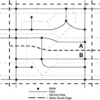
• The equal flow distribution option simply divides the known flow evenly between the demand nodes. The equal flow distribution strategy is illustrated in the diagram below. The lump-sum area in this case is a polygon layer that represents meter route areas. For each of these meter route polygons, the total flow is known. The total flow is then equally divided among the demand nodes within each of the meter route polygons (See Figure).
• The proportional distribution option (by area or by population) divides the lump-sum flow among the service polygons based upon one of two attributes of the service polygons-the area or the population. The greater the percentage of the lump-sum area or population that a service polygon contains, the greater the percentage of total flow that will be assigned to that service polygon.

Each service polygon has an associated demand node, and the flow that is calculated for each service polygon is assigned to this demand node. For example, if a service polygon consists of 50 percent of the lump-sum polygon's area, then 50 percent of the flow associated with the lump-sum polygon will be assigned to the demand node associated with that service polygon. This strategy requires the definition of lump-sum area or population polygons in the GIS, service polygons in the model, and their related demand nodes. Sometimes the flow distribution technique must be used to assign unaccounted-for-water to nodes, and when any method that uses customer metering data as opposed to system metering data is implemented. For instance, when the flow is metered at the well, unaccounted-for-water is included; when the customer meters are added together, unaccounted-for-water is not included.

In the following figure, the total demand in meter route A may be 55 gpm (3.48 L/s) while in meter route B the demand is 72 gpm (4.55 L/s). Since there are 11 nodes in meter route A, if equal distribution is used, the demand at each node would be 5 gpm (0.32 L/s), while in meter route B, with 8 nodes, the demand at each node would be 9 gpm (0.57 L/s).

Point Demand Assignment

A point demand assignment technique is used to directly assign a demand to a demand node. This strategy is primarily a manual operation, and is used to assign large (generally industrial or commercial) water users to the demand node that serves the consumer in question. This technique is unnecessary if all demands are accounted for using one of the other allocation strategies